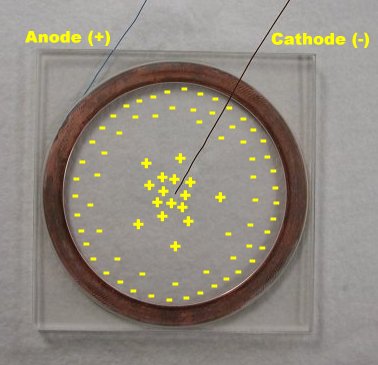
Electro deposition means to deposit a dissolved or suspended substance onto an electrode by electrolysis. In our case, copper is dissolved in an aqueous copper-sulfate solution of a known concentration. Electrolysis splits the CuSO4 molecule and Cu++ ions are deposited on the cathode.
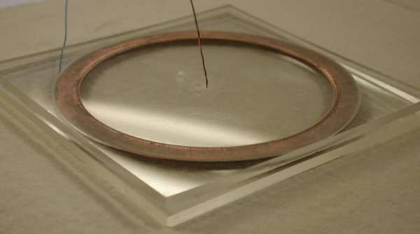
We used a lathe to etch a circular groove about 0.5 mm deep, centered on one of the Plexiglass plates. This groove is where the copper ring will sit and thus has the same inner and outer diameters. Since the groove is only 0.5 mm deep and the ring is 1 mm thick, when the ring is in the groove, it will protrude 0.5mm leaving a cavity where aqueous CuSO4 can be poured. This same plate had a small hole drilled in the center, just big enough for the un-insulated copper wire to be inserted. In hind-sight, it would have been better for the groove to be in one plate and the hole in the other in order to facilitate the setup of the experiment (see below).
The copper ring will serve as the cathode. Thus, we needed a way to attach the ring to a power source. Soldering to the copper ring was not as easy as it might seem. We had a difficult time getting a good connection between the wire and the ring. During the period of the growths I had to re-solder the wire about three times. So it is important to make a good connection between the wire and the ring and this is accomplished by carefully preparing the surface.
First, a sharp blade was used to scrape the surface of the ring until it was nice and shiny. This is to remove any oxidation and gives the surface a bit of a rough texture. Using fine grained sandpaper would probably work even better. Once that is done, use the soldering iron to heat the surface and then use some acid flux and coat the surface. Once that is done, use a small amount of solder and coat the surface, rubbing over the solder many times until it is flat. This is called "tinning". Finally, you're ready to apply the wire. Just rest the wire on the surface and move the solder around until the wire attaches. You may need to add a bit more solder.
It is helpful to use a vice to hold the ring in place and make sure you use a nice, hot iron with a large, flat tip. I used 28 guage wire (wire-wrap wire) and soldered it to the side edge of the ring. If you put it on the top edge, the ring will not rest flatly in the groove of the Plexiglass plate.
We started with a copper-sulfate powder, CuSO4-5H20. CuSO4 has a formula weight of 159.6096 and 5H2O of 90.077. Thus, when making an aqueous solution, you must take into consideration the water already present in the powder where 1 gram of H2O corresponds to 1 mL.
For an aqueous solution of copper-sulfate with a concentration of 1 molar (1 M), you need 1 mole of CuSO4 to 1 liter of water (1 m CuSO4/ 1 L H2O). Thus, you would need 159.6096 + 90.077 = 249.6866 grams of copper-sulfate powder mixed with 1 L – 90.077 mL = 989.933 mL H2O. In all cases, we used de-ionized water and a magnetic mixing device. Just mix the solution until it is homogeneous, usually around 10 minutes.
Our solutions ranged from about 0.01 M to 0.3 M. It is believed that saturation lies within that range because the higher concentrations had an orange substance settle after a period of time. It is guessed that the substance was copper and thus we made sure the solution was well shook before beginning the experiment.
We used a Sony Camcorder with resolution 720 X 480 to do time-lapse video recordings of the growths. Some of these are availble for download below. We also took pictures with a Nikon Coolpix digital camera with resolutions as high as 2048 X 1536.
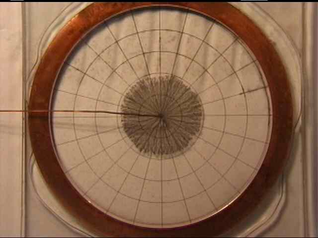
To start a simulation, you simply place the copper ring on the bottom Plexiglass plate and carefully pour the solution into the center of the ring. Then, carefully lay the grooved Plexiglass plate on top such that the copper ring fits into the groove. As mentioned above, it would probably be better to have the groove on the bottom plate and the drilled hole in the top plate. But our setup does work and once you have the top plate on, carefully insert the wire into the drilled hole.
Attach the wires to a power source and get the camera equipment set up. We used a nice, heavy tripod leaned against a workbench. Finally, apply a voltage while simultaneously starting the time-lapse recording and a stopwatch. Different growths grew at different rates and thus the interval between video snapshots changed.
| C o n c e n t r a t i o n (M) |
| ||||||||||||||||||||||||||||||||||||
| Voltage |
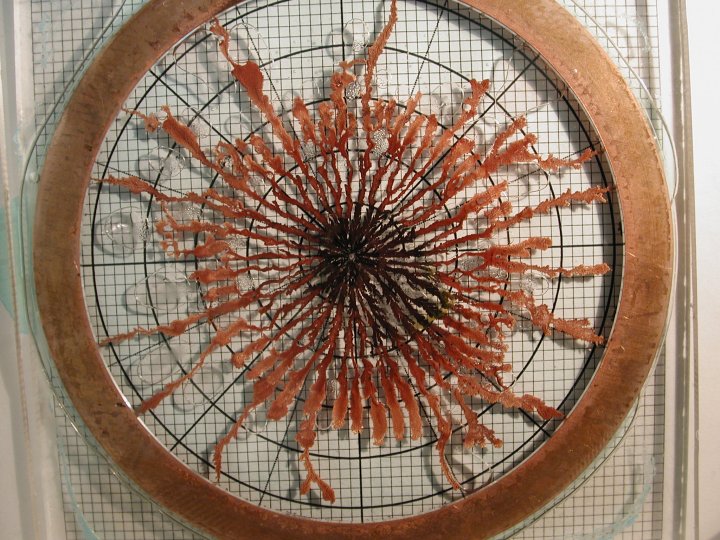
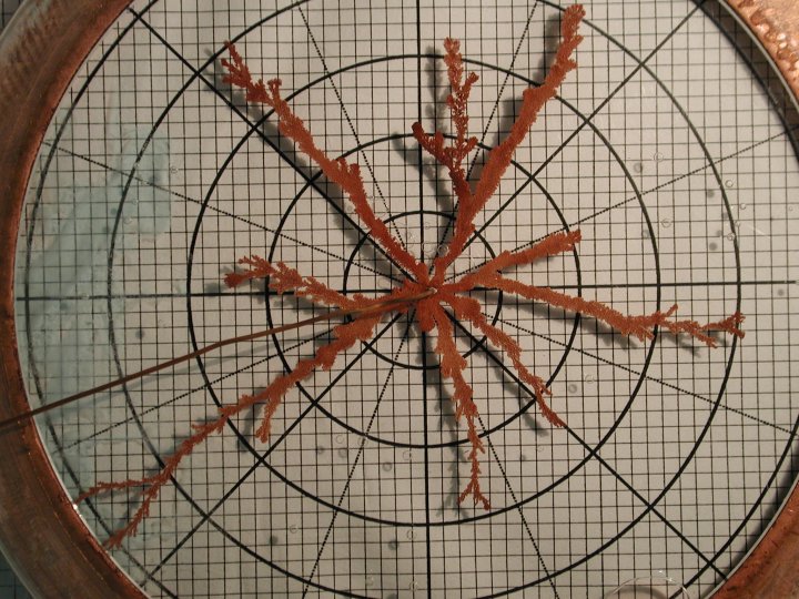
The above table gives a general overview of the aggregates we grew. Notice how changes in concentration and voltage greatly effect the type of pattern realized. Low concentrations lead to highly dense structures across many different voltages. As the concentrations increase, we notice a greater senesitivity to changes in voltage where instabilities tend to select out branches.
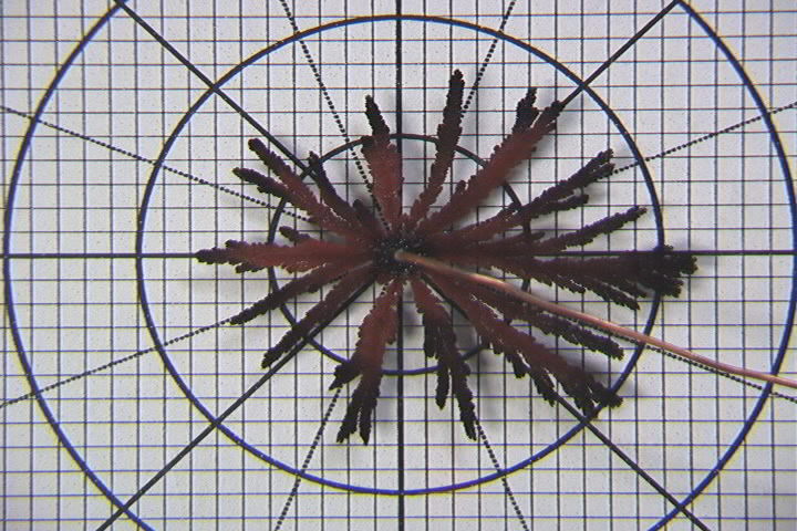
| 0.2M, 4 Volts | |||
 |
 |
 |
 |
| 3 | 2 | 2 | 2 |
| 0.2M, 8 Volts | |||
 |
 |
 |
 |
| 8 | 9 | 7 | 8 |
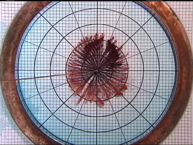
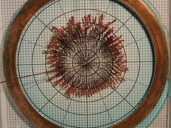
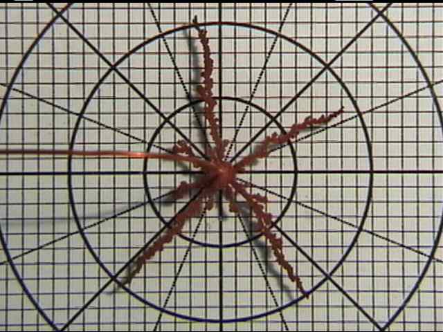
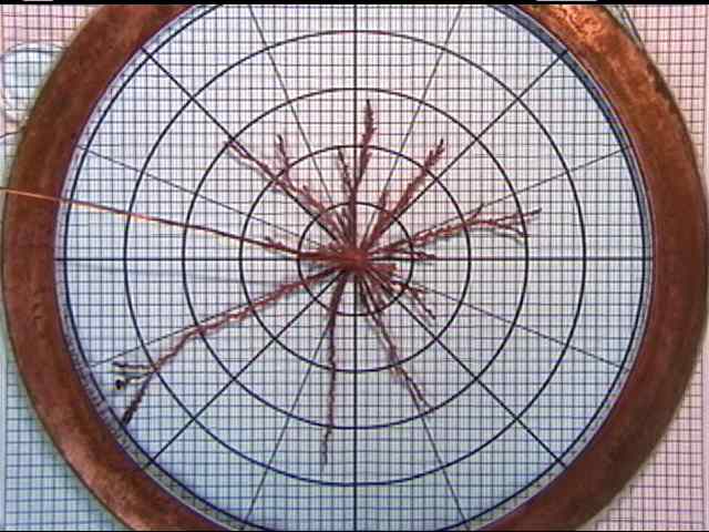
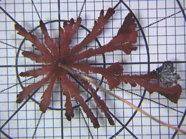
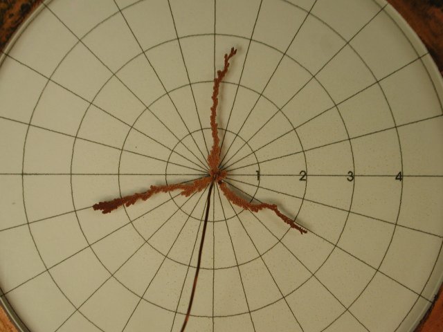
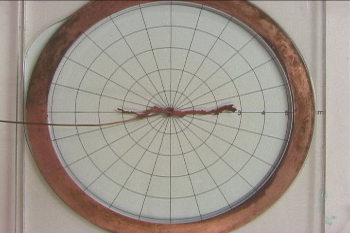
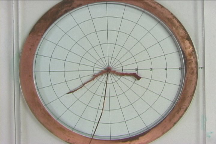
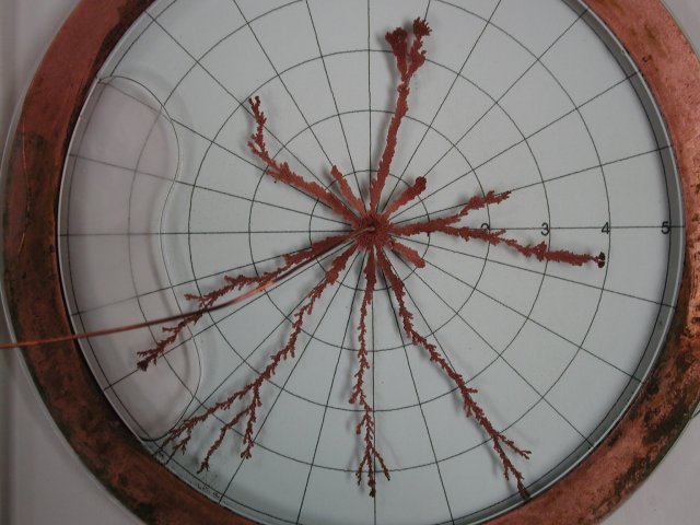
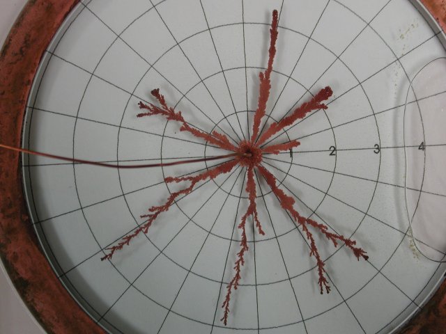
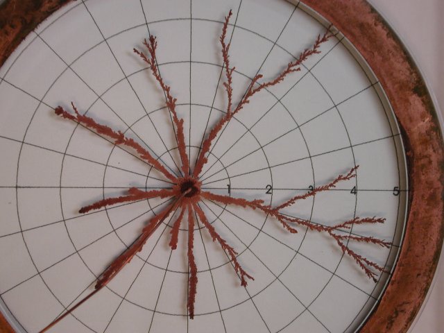
All of the above aggregates were created from a 0.2M solution, the top row driven at 4 volts and the bottom row driven at 8 volts. The number beneath each image is the number of branches counted at a radius of 2 cm. We can see that the types of patterns formed are indeed reproducible. However, one might wonder if there is a certain solution concentration and voltage where the reproducibility would fail.
| 0.3M with Magnetic Field | /0.3M6V(M).jpg) |
/0.3M8V(M).jpg) |
/0.3M10V(M).jpg) |
/0.3M10V(M)B.jpg) |
| 6V | 8V | 10V | 10V |
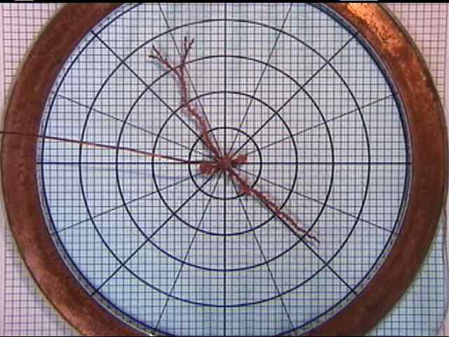
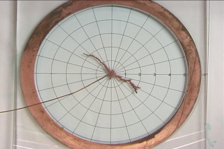
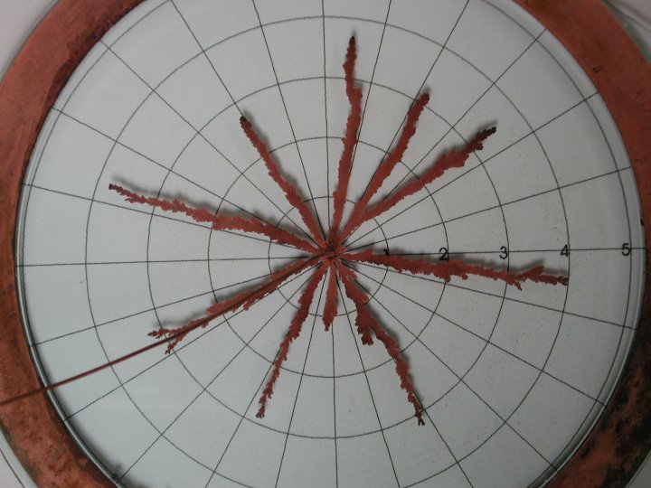
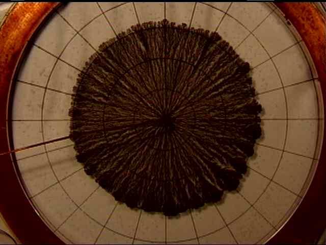
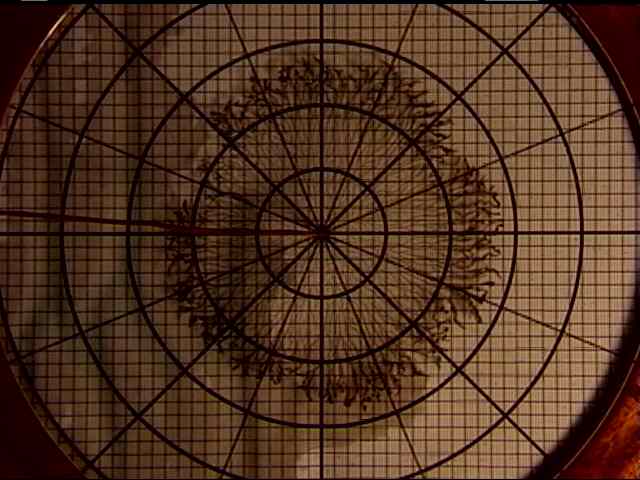
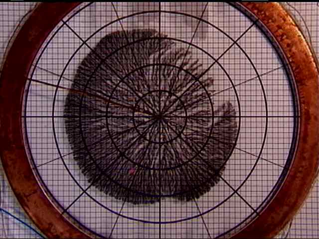
All the growths above were created from 0.3 M concentration of CuSO4. This time a magnetic field was applied by placing a magnet underneath the electrodeposition cell. The electric field causes the Cu++ atoms to have a velocity towards the center of the cell. These moving charges interact with the magnetic field causing a Lorentz force in the clockwise direction.
Of course, you can see that different magnets were used in different orientations. The two left-most growths had identical magnets placed 120 degrees apart and 2 cm from the center. You can see that there was little change in the growth between the two. However, if you compare them to the 0.3 M 6 and 8 volt growths above (with no magnet), you can see a big difference in the type of pattern. I am not convinced that this is due to the magnetic field, but perhaps due to the plate separation which had changed during the course of these experiments.
The plates warped in such a way that they were no longer flat, but curved or concave. Luckily, they warped in the same direction, but in some in cases where the magnetic field was applied, I had not noticed this. I am fairly certain that the plates were misaligned in these cases. One plate was probably concave up while the other was concave down. Thus, the plate separation was greatly reduced. As a remedy, the plates were aligned such that they had the same orientation and then small scratches were made in one corner. This way the plates could be aligned the same way in each run.
The third growth from the left had just one magnet, the same used in the 6 and 8 volt cases, but placed directly in the center. Finally, for the right-most growth, we used a much larger and more powerful magnet. Its effects are easily noticed.
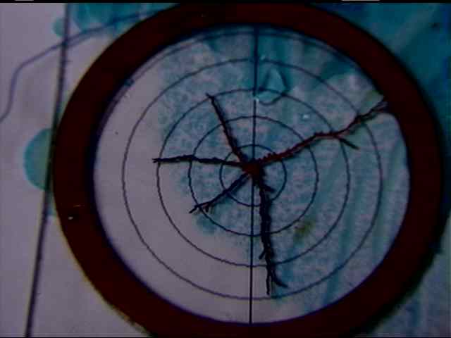
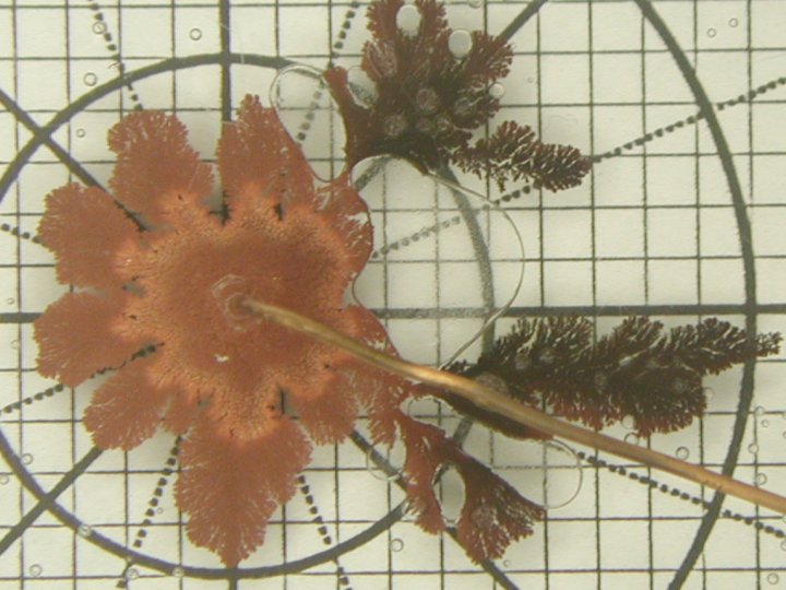
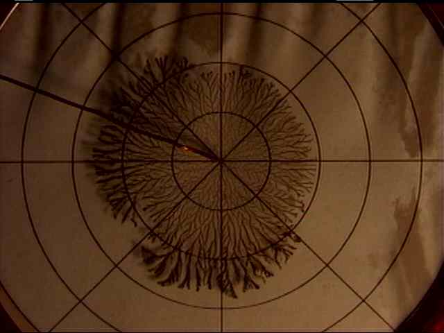
The copper ions drift towards the cathode and upon reaching the cluster are reduced and stick. At the beginning of this process, the atoms conglomerate in a bumpy fashion. The electric field is stronger on the bumps and thus the copper ions are more strongly attracted to them. As the bumps grow, the electric field at the tips grows. It is this interplay between the microscopic Cu atoms moving randomly about and the macroscopic electric field that causes the many patterns we see.
Also, the anisotropy of the copper is necessary for some types of patterns to occur. This is why it has been suggested to use a zinc-sulfate solution because its anisotropy is more pronounced. There have been studies using ZnSO4 where the types of patterns formed were grouped into four basic morphologies: DLA, dense radial, dendritic, and needle crystal [3]. If a plot is made of solution concentration versus voltage, it can be demonstrated that there are regions in the plot where only one type of pattern is realized and other regions which are transitional regions where two or more different types of patterns are noticed.
0.01M, 2V
0.01M, 4V
0.01M, 6V
0.01M, 8V
0.01M, 10V
0.1M, 2V
0.1M, 4V
0.1M, 6V
0.1M, 8V
0.1M, 10V