Diffusion Limited Aggregation, or DLA, was first introduced by Tom Witten and Len Sander as a model for irreversible, colloidal aggregation [1]. However, it was soon realized that the model could be used in many different applications. The basic idea is to let a particle move about under Brownian motion. If the particle moves to a location with a nearest neighbor, it sticks. The patterns which emerge from this simple model are astounding.
More specifically, to simulate this model on a computer, you initially set a two-dimensional array (other dimensions could also be used). In our case, this array can be looked at as an n X n grid. I used grid sizes of 1000 X 1000 (n=1000) and 300 X 300 (n = 300). The grid is initialized to "0" with the (n/2,n/2) location set to some value determined at run time. This value, call it the potential, denotes the presence of a particle.
Once the grid is initialized, another particle is introduced at a random point on a circle of radius r+dr, where r is the maximum radius of the growth and dr is just some small increment. Then, let it move randomly in any of four Cartesian directions: up, down, left, right. Three things can happen at this point. 1) The particle moves sufficiently far away that it is discarded and a new particle is introduced, 2) the particle moves to a location with a nearest neighbor and sticks, or 3) the particle moves to a location with no neighbors and thus is randomly moved again.
The first situation might need a little explaining. You may wonder how a particle could disappear and then reappear in some random location, but actually that is not what is happening. Two things can happen when the particle moves far away. Either it moves infinitely away and thus we do not care about it and introduce a new particle, or it moves out of bounds and eventually diffuses back into the growth area at some random location, which is what we assume. As a matter of fact, to decrease run-time, we generally set the “far away” limit at some radius, r + dr' where dr' > dr. In a sense, we are picking out only the particles that stick. We are not concerned with particles that diffuse far away from the growth.
To see DLA in action, check out Diffusion Limited Aggregations (a fractal growth model). This java applet will allow you to watch the clusters grow in real-time.
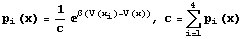
The method just described is what is known as DLA. However, since we were attempting to model electrodeposition, we needed a way to include the drift caused by the electric field. To do this, we note that the potential satisfies Laplace’s equation. So every time a particle is added to the growth, we calculate the potential at every point on the grid and use this to determine the probably of moving in a particular direction, where the probability to move in the ith direction is,
To make this model even more realistic, you could write in a way to control the concentration [9].
Inputs for each run are the potential (the potential at the growth), beta (the probability constant shown above), and id and od which are the spawn and kill radii, respectively. Also, you can change the size of the grid, n, and the number of particles to introduce, iterations. However, all of the clusters shown here had grid sizes of 300 X 300 and introduced enough particles that the cluster reached the edge of the grid.
To calculate the potential at each point of the grid, we simply took the average of the potentials of each nearest neighbor. The more times you perform this operation, the more accurate the approximation. In my growths, I calculated the potentials at each point every time a particle stuck to the cluster and performed the averaging square-root of r times, where r is the maximum radius of the cluster. In other words, if the maximum radius of the cluster were 150 particles at the time a new particle stuck, I would average the potential at each point on the grid twelve times. Which is to say, average the potential at each point, then do that again, and again, twelve times.
One could speed up the process by performing the potential calculation say, every 10 or 20 particles, but since my grid sizes were only 300 X 300, it did not slow the simulation too much by performing the calculation every time a particle stuck.
C++ code: DLA.zipOf course, one thing you may be wondering is exactly how do you move a "particle" randomly using a computer. It would seem that any way you can think of to generate a random number using a computer would be deterministic, and indeed, it is. The random number generator I used was suggested by D.E. Knuth [3]. For a given seed, the algorithm will generate the same sequence of numbers every time. Are they random? What is random?
Two tests I made to check that the numbers were random was to take each successive pair and plot them with the first number representing the x coordinate and the second number representing the y coordinate. The points were randomly spread throughout the plot, looking something like static on a television set. The other test I performed was to bin the numbers and create a histogram. The histogram showed that there was not a particular number more likely to occur than another.
These tests are not exhaustive and the number generator I used is not the most sophisticated, however, it produced numbers which were “random enough” for our purposes.
One of the principle concerns when looking at these patterns is finding some way to group them. We know that one pattern looks different from the other, but exactly how? One measurement you can perform is to find the box-count dimension [4]. The box-count dimension is a type of fractal dimension and is a measure of the roughness of the boundary. You simply break the grid up into equal squares and count the number of squares which include a boundary. Then you break the grid up into a different number of equal squares and count the number of those with a boundary. If you think of the number of squares which contain a boundary as a measure of the length of the boundary, then you can see that the smaller the squares become, the more accurate the measure of the length of the boundary. The box-count dimension is a measure of how this length changes with greater and greater resolutions.
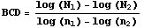
N is the number of squares with a boundary and n is the total number of squares the grid was broken up into.
|
|
|
|
|
|
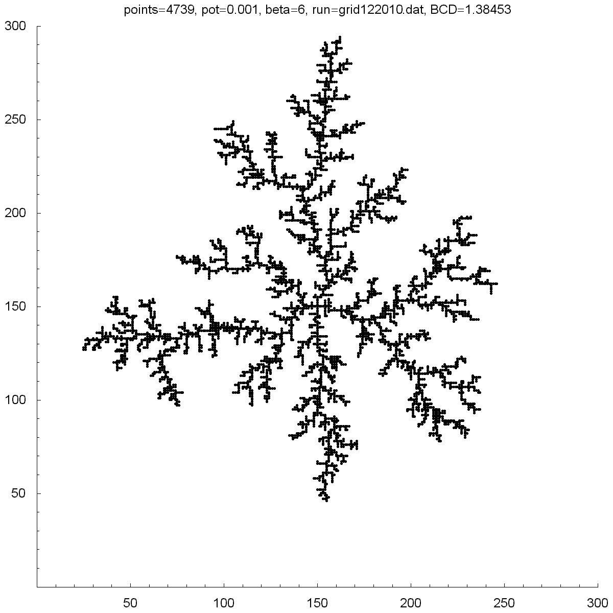
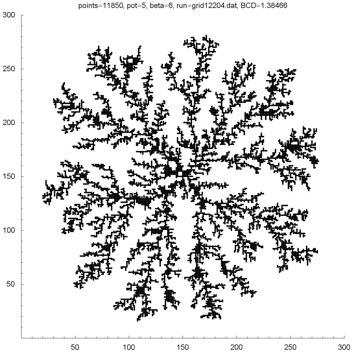
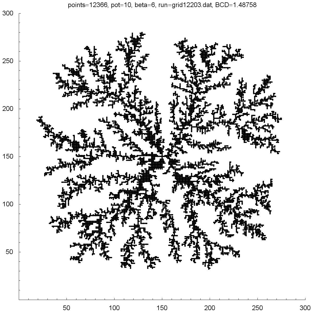
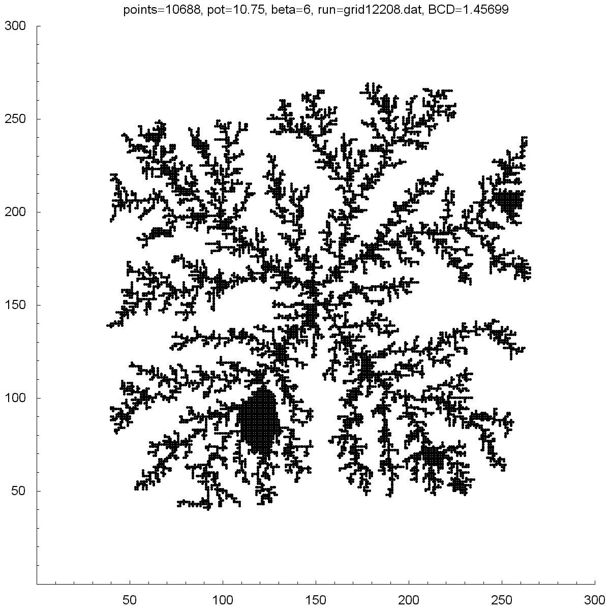
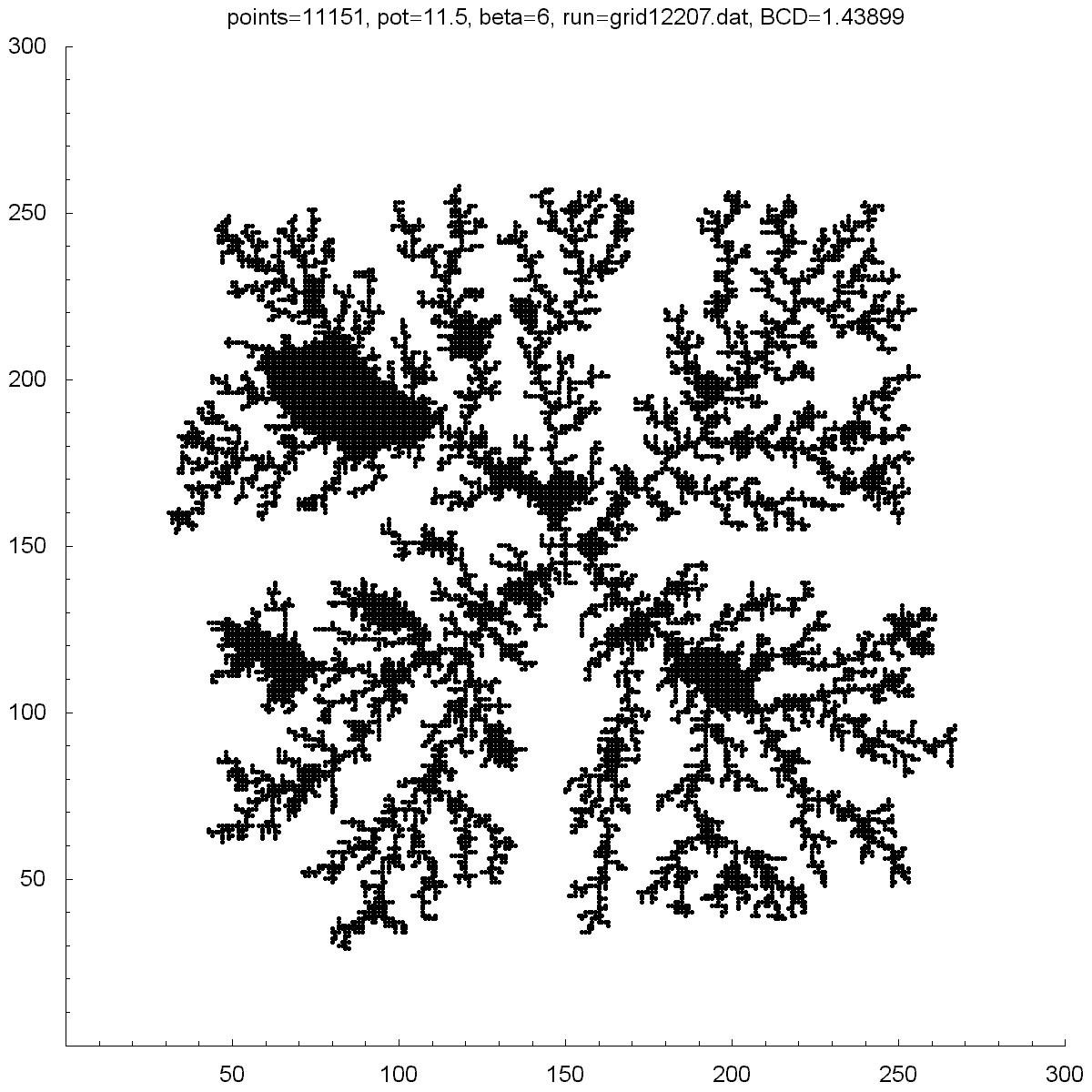
| Potential | 0.001 | 5 | 10 | 10.75 | 11.5 |
| BCD | 1.38453 | 1.38466 | 1.48758 | 1.45699 | 1.43899 |
| Points | 4379 | 11850 | 12366 | 10688 | 11151 |
|
|
|
|
|
|
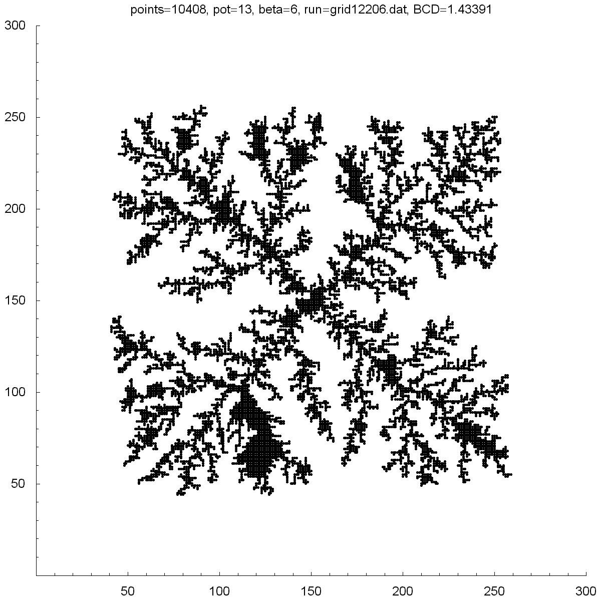
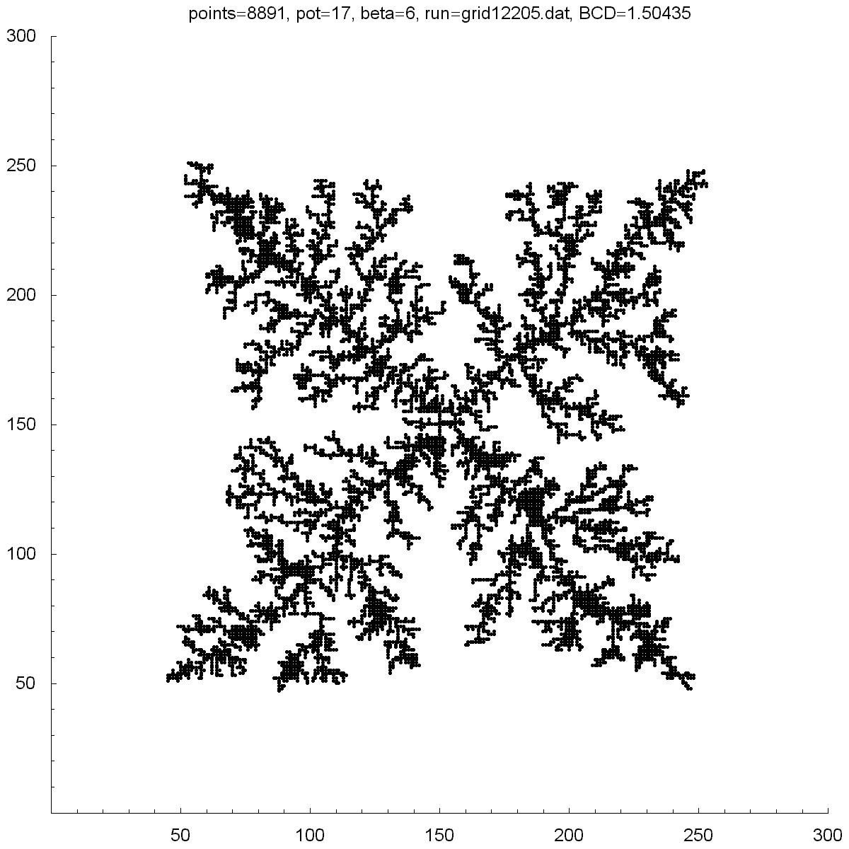
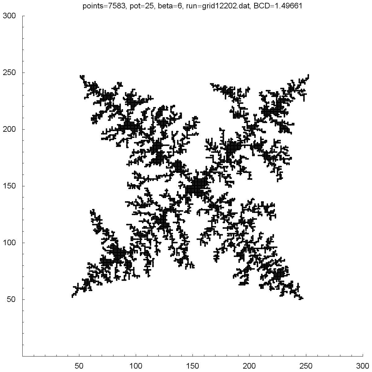
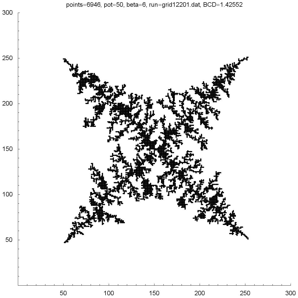
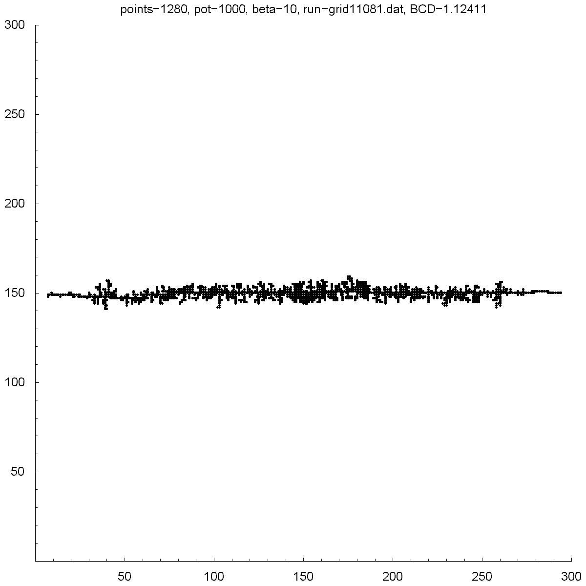
| Potential | 13 | 17 | 25 | 50 | 1000 |
| BCD | 1.43391 | 1.50435 | 1.49661 | 1.42552 | 1.12411 |
| Points | 10408 | 8891 | 7583 | 6946 | 1280 |
All of the clusters above were created with DLA.cpp. In each case beta was set to 6, except for the bottom-right cluster which had a beta of 10. Underneath each picture is the value at the which the potential was set to, the Box-count dimension (BCD) measured for each case, and the number of points (or particles) in each cluster. You can see there is a transition region between potentials of 10 and 50 where the BCD reaches a maximum.
You can also notice how, as the potential is increased, the clusters tend to branch towards the four corners. I do not know why this occurs as one would guess the branches would grow towards the four sides where the calculated potentials would be highest.
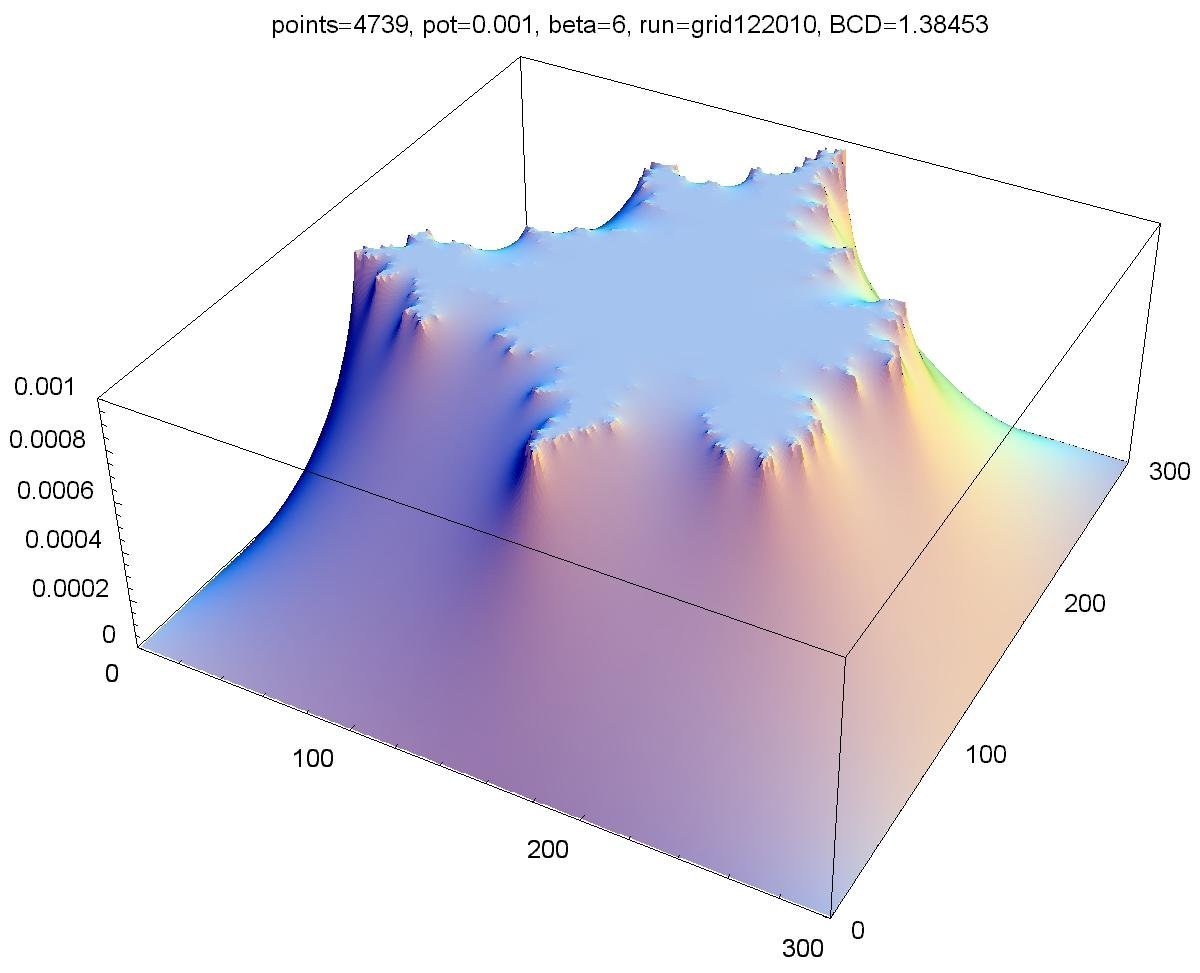
Above is a plot of the potentials at each point on the grid for a potential of 0.001 (see upper-left image above). You can see on the vertical axis that 0.001 corresponds to points on the cluster and zero corresponds to the boundaries. Since the probability to move in a particular direction was proportional to the gradient of the potential, you can see that the particles were much more likely to move towards a tip of the growth. It was very unlikely for a particle to move deep into one of the fjords of the growth.